RAIRD Information Model (RIM)
Version 1.0 16^th June 2014
RAIRD P 1.1 Information Model
Authors: Jenny Linnerud SSB, Ørnulf Risnes NSD, Arofan Gregory MTNA
Approvals

Change log

This work is licensed under the Creative Commons Attribution 4.0 International License. To view a copy of this license, visit http://creativecommons.org/licenses/by/4.0/. If you re-use all or part of this work, please attribute it jointly to Statistics Norway and the Norwegian Social Science Data Services.

Contents
1. Introduction
2. RAIRD Information Model (RIM)
2.1 RIM Design Principles
2.2 Extending the model
2.3 Notation
3. System Overview
4. Input Data and the Event History Data Store
4.1 A Simple Example
4.2 GSIM Unit Data Structure
4.3 Datum-Based Data Structure
5. Analysis Data Sets
5.1 GSIM and Unit Data
5.2 Analysis Data in RIM
6. Provisional and Final Outputs
6.1 RAIRD Requirements
6.2 The GSIM Dimensional Data Model
7. Topics and Concepts for Organization of Data
7.1 Requirements for Topic and Variable Navigation
7.2 GSIM – Mapping to RIM Requirements
7.3 Administrative Details
8. Concepts, Classifications, Variables and Related Metadata
8.1 Concepts
8.2 Units, Unit Types, and Populations
8.3 Variables
8.4 Value Domains, Statistical Classifications, and Codelists
9. Disclosure Control Rules and Risk Minimization Actions
9.1 GSIM and Disclosure Control
9.2 RIM Model
10. Process Descriptions
10.1 The GSIM Process Model
10.2 Load Event History Data Store Process
10.3 Interact with the Virtual Research Environment Process
10.4 Control of Disclosure Risk Process
10.5 Accredit Institutions and Manage Users Process
i)    Standard users
ii)   Specific, large users
iii)  Institutions with special requirements within health registers
iv)  Students
11. References
List of Figures
Figure 1: System Overview
Figure 2 Unit Data Structure
Figure 3: Datum-based Data Structure
Figure 4: Populations and Units
Figure 5: Unit Relationships
Figure 6: Data Sets
Figure 7: Concept
Figure 8: Population
Figure 9: Variable and Represented Variable
Figure 10: Instance Variable
Figure 11: RIM Represented Variable extension
Figure 12: Node
Figure 13: Disclosure Risk Assessment
Figure 14: Disclosure - Corrective Actions
Figure 15: Design Processes
Figure 16: Run Process
Figure 17: Accredit Institutions and Manage Users Process Flow
Figure 18: Accreditation
Figure 19: Researcher Access Request

Introduction

There is an increasing demand for access to micro data from researchers and for empirical research based on register data from public government. For register data this user demand has to be met in a way that is in accordance with the principles of data protection and confidentiality for micro data. These principles of confidentiality are normally legal founded and are common for official statistics in most countries.
In Norwegian official statistics there is wide use of administrative data. Statistics Norway also has close cooperation with administrative registers like the Population Registers and Central Coordinating Register for Legal Entities. The common identifiers (persons and economic units) give Statistics Norway the possibility to link information from different sources (administrative and own statistical surveys). Data with identifiers are stored and accumulated over time. The data may be combined and presented as cross section data. Data may also be combined in ways that give longitudinal data.
Statistics Norway and the Norwegian Social Science Data Services (NSD) aim at establishing a national research infrastructure providing easy access to large amounts of rich high-quality statistical data for scientific research while at the same time managing statistical confidentiality and protecting the integrity of the data subjects. The work is organized as a project, RAIRD – Remote Access Infrastructure for Register Data ¹ , and funded by the Research Council of Norway.

RAIRD Information Model (RIM)

One of the first deliverables in the RAIRD project is the RAIRD Information Model (RIM) v1.0.
An information model (IM) is an abstract, formal representation of objects that includes their properties, relationships and the operations that can be performed on them. The main purpose of RAIRD IM (RIM) is to model managed objects at a conceptual level, independent of any specific implementations or protocols used to transport the data.  The degree of specificity (or detail) of the abstractions defined in the RIM depends on the modelling needs of its designers.
RIM is an implementation of the Generic Statistical Information Model (GSIM) v1.1. It is extending GSIM to include the users (producers, administrators and researchers), but does not include parts of GSIM that we consider to be more related to the details of the official production of statistics, e.g. Change Definition, than to the secondary use of the microdata by researchers.
We have used GSBPM as a tool to discuss which parts of the statistical production process could also be of relevance for researchers using RAIRD. For example, the build and collect phases will not be necessary for the researchers as the RAIRD system will be provided by Statistics Norway and the data are already collected by us. RAIRD will need to heavily support the Specify needs, Process and Analyse phases for the researchers.
This document is aimed at metadata specialists, information architects and solutions architects.
There are also a number of annexes, which include a glossary (including relevant GSIM information objects), relationship between RAIRD and business process models, a technical overview of information flows and a mapping to DDI.

2.1 RIM Design Principles

The design principles for RIM listed below are based on the design principles in GSIM v0.8 and the design principles for DDI.

2.2 Extending the model

One of the RIM design principles is that RIM can easily be adapted and extended to meet users' needs. It is expected that implementers may wish to extend RIM during the RAIRD project, by adding detail and indicating which information objects are used, and exactly how.
RIM itself should be used as an example of how to document extensions and restrictions. This means providing the information in the template found in the GSIM v1.0 Specification and providing the definitions and descriptions/examples in this tabular form, as well as providing an overall narrative of each UML diagram produced. 

2.3 Notation

Throughout this document we have used the following notation:

• The Names of GSIM information objects start with a capital letter and are written in italics e.g. Unit Data Set
• The Names of RIM information objects, that are not GSIM information objects, start with a capital letter and are written in bold italics e.g. Provisional Output
• The Names of systems and processes in RAIRD start with a capital and are written in bold e.g. Event History Data Store and Interact with the Virtual Research Environment Process.

System Overview

The RAIRD Information Model (RIM) is intended to support all aspects of the RAIRD implementation. In order to understand this scope, a basic understanding of the systems and processes in RAIRD is helpful. In the illustration below, the major systems and information flows in RAIRD are visible:

Figure 1: System Overview
We will briefly describe each of the systems and information types presented above. We begin by describing how the data is provided to RAIRD. The SSB Data Management System is external to RAIRD – all other systems and information flows are part of the overall RAIRD application.
There will always be some system or systems for managing the collection, production, and dissemination of statistical data and metadata within SSB (SSB Data Mgt. System). These systems are liable to change over time, driven by the various needs within the organization. Consequently, an API will be created specifying how the data and metadata used by RAIRD should be supplied (Load API).
Two types of information will be supplied through this interface: the data itself (Event History Input Data Set), and the relevant metadata (Input Metadata Set). The data could be supplied as a delimited ASCII file in a form roughly similar to how it will be stored in the receiving system. The metadata could be transmitted in a standard format, such as DDI. ² This information would be loaded into the Event History Data Store, where it would be placed into a system capable of handling the very large numbers of records and serving them up in a performant way. It should be noted that the structures of the data inside the store and in the data-loading format could be quite similar, consisting of a simple datum-based data structure (see section 4.3). ³
The store contains the information needed by the users to formulate meaningful requests, including some calculated information such as for what time periods data is present for specific variables.
Having loaded the needed information into the storage system, the researchers now enter the picture. Researchers will be associated with accredited institutions that have applied for access to RAIRD, and will have been given necessary training on how to properly use RAIRD. The users will be given access to the system, but they and their institutions are held liable for any misuse of the system or the confidential data contained. The entire process of institutional accreditation and the management of users and access to the system are part of the system and therefore the RAIRD Information Model, but they are not shown in this particular diagram.
Users will access RAIRD using a browser-based anonymizing interface, loaded from the Data Catalogue, which exposes the contents of the Event History Data Store using the metadata held in it. The researcher can browse the available variables (grouped topically according to a set of concepts), see possible unit types of study, the time period for which variables are available, and similar descriptive aspects of the data. The researcher is thus able to familiarize themselves with the data available to answer any specific research question, but will not see microdata.
The researcher will look at the data within a conceptual framework that does not reflect the actual structure of the Event History Data Store, but allows them to think about data selection using the format in which it will be extracted (eventually, the Analysis Data Set). This data structure is one that is very familiar to researchers, as it is the one which is most often used within statistical packages such as SAS, SPSS, Stata, and R.
The RAIRD Virtual Research Environment (the browser-based interface) now allows the researchers to perform their data selection, processing, and analysis. User Operations are performed through browser-based interactions with the Virtual Statistical Machine. The operations specified by the user are logged, so that there is a clear audit trail. (RAIRD will have the capacity to re-create any researcher action accurately, by re-executing the function on the correct version of the data store, for which any changes are also logged.)
Researchers are able to select data by specifying one or more variables they wish to process, and by specifying a point in time for which they want the variables populated. If event-history processing is desired, a time period may be specified for variables of interest, so that changes across time can be seen. Note that having more event variables at a time in an analytical data set will result in a non-uniform unit identifier. Measures must be taken to communicate this complex structure to users. Such communication techniques are not yet defined. Note also that data sets with multiple event variables cannot be analyzed using the same techniques as data sets with a well-defined unit identifier. Analysis techniques for working with multiple event-based variables have been defined as outside the scope of the first versions of RAIRD. The latter type of variable is termed an event history variable, and the others are termed static variables. The Unit Type for each variable is known – the selected data is presented to the researcher for analysis using the finest grained unit from the selected variables. The selected data is the Analysis Data Set. Additional processing may now be performed on this data set, which can be supplemented by additional data selection as needed. The researcher can generate new variables from the old ones, reshape the data set, perform cleaning and validation, and other types of processes.
The data analysis is based on statistical functions (tabulation, regression, etc.) executed by the Virtual Statistical Machine on the Analysis Data Set. The result of this is a Provisional Output,. The researcher does not see this Provisional Output – first, it is scrutinized by the Disclosure Control Engine, which executes a set of operations to guarantee, to the extent possible, that it is not disclosive, according to the criteria established by Disclosure Control Rules. Rules might cause corrective actions to be applied until the Provisional Output meets all desired criteria. At this point the corrected Provisional Output is passed to the researcher as a Final Output, which again appears in the browser interface. The researcher might wish to re-run further statistical functions on the Analysis Data Set, or might go and try a different selection of data altogether. This process continues until the researcher has the desired results.
GSIM Coverage
Note that there are three very different – but related – types of data structures in this process. The data loaded into RAIRD has a very event-history-based structure, with a single datum recorded for each available event. The Analysis Data Set has a different structure, organized into traditional rows and columns – what GSIM calls a Unit Data Set. The results of statistical operations may be tabular, but more typically as estimates of statistical model parameters and graphical displays – what GSIM describes as a Presentation. The RAIRD Information Model describes all of these, using what GSIM offers, but extending it to cover event-history data.
Further, we have many different examples of processing: the loading process, data catalogue browsing, data selection, data processing, data analysis, and the application of disclosure control. These processes will be modeled using the information objects supplied by GSIM.
Other functions (institutional accreditation, user management) are not as well-described in GSIM, and will require RAIRD-specific extensions.

Input Data and the Event History Data Store

This section attempts to explore the datum-based modeling of data using a simple example, and contrasts this with the similar way in which data can be described using the unit data model found in GSIM. The goal is to provide a good basis for discussing and integrating the RAIRD datum-based approach with the GSIM model, since the RIM will – wherever fit for use - be based upon it.
The datum-based model is one which is similar to some styles of data warehouse design, in which each single fact has a set of descriptors, using a star schema approach. It is not, however, necessary to use this approach with the datum-based model, and there are potentially large differences from an implementation perspective. Like the fact in the star schema approach, the individual datum is central to how we conceptualize the data structure.
In GSIM unit data, the conceptual model is more similar to the structure of relational database tables: each record is associated with a single unit, and provides a set of values for a known sequence of variables.

4.1 A Simple Example

We will use a very simple example as the basis for comparing the two styles of data modeling (the GSIM unit data approach and the RIM datum-based approach).
We have a variable marital status, represented with the following codes:
N - single and never married
C - cohabitating and never married
M - married
S - separated
D – divorced
For our example, we have an identifier of 0937, which identifies an individual. This individual was married on August 4, 2003, and remains married.

4.2 GSIM Unit Data Structure

In a Unit Data Set, the value for marital status would appear as a column in a table, typically alongside several other variables describing the individual 0937. We can visualize this as shown in the table below.

Here, we have first the case identifier (CASE_ID), then a date of birth variable (DOB), followed by our marital status variable (MAR_STAT), gender (GENDER), the date married (DATE_MAR), date separated (DATE_SEP), and date divorced (DATE_DIV). Note that the latter two variables have null values, as individual 0937 is still married. We see this by the code found for the marital status variable, M. Of course, any individual could have multiple marriage/separation/divorce events.
There are other ways of encoding data modeled as GSIM unit data, but this example is fairly typical – in implementation, the data could be stored in relational database tables structured as shown, stored in fixed-width or delimited ASCII files (such as CSV), or stored in this form in statistical packages such as SAS, Stata, SPSS or R.
GSIM models this in a fashion that places emphasis on the Logical Record: the sequence of variables associated with each Unit (as expressed by our Case ID above). In the GSIM model, we have the following diagram:


Figure 2 Unit Data Structure
[Source: Part of GSIM Specification v1.1 Figure 19]
The Unit Data Set is structured by a Unit Data Structure, which has at least one Logical Record. This Logical Record provides the structure for the Unit Data Record, which groups Unit Data Points. To translate our example, each value in our table is a Unit Data Point. These are grouped into a row: the Unit Data Record. Each Unit Data Record (row) – the sequence of variables repeated throughout the file - is structured by the Logical Record, which describes a type of Unit Data Record for one Unit Type within a Unit Data Set. Although not shown in this diagram a Logical Record groups Data Structure Components that group Represented Variables.
GSIM tells us that Represented Variables may play three roles as Data Structure Components: Identifier Components, Measure Components, and Attribute Components.
In our example, each value (0937, 1971-05-03, M, 1, 2003-08-04,,) is a Datum – the GSIM structural description of the position occupied by each Datum is a Unit Data Point. When we group these together, they become a Unit Data Record. The Logical Record then tells us that the first value is an Identifier Component and all the remaining variables are Measure Components.

4.3 Datum-Based Data Structure

In our datum-based model, we have only a single Datum (value) in our conceptual row (that is, there would be a separate row for each variable value):

The case identifier (CASE_ID) is needed for each entry because we need to be able to associate the value with the Unit (Individual 0937). The variable reference (VAR_REF) is needed because we need to know which variable (MAR_STAT) is associated with the value. The value (VALUE) is obviously needed. The start and end dates (START_DATE, END_DATE) are needed in the case of event history data – for snapshot data we need only a single date, the time of observation. Because individual 0937 could potentially become separated or divorced, etc., we would also need to be able to record the dates of any changes in marital status.
Many of the conceptual objects we need to describe this structure exist in GSIM: we have the idea of a case identifier variable (it is an Identifier Component); we have the Represented Variable object to which we can make reference; we have the idea of a Data Point.
It is worthwhile at this point to illustrate what the entire row of our example data would look like when modeled according to the datum-based approach:

Notice that the date variables – DATE_MAR, DATE_SEP, and DATE_DIV are no longer needed, as their contents are carried in the start date and end date columns, in combination with a change in marital status. DOB is a bit strange, because the value is a fixed one which cannot change. Still, the event remains consistent as shown. This is because every datum is given a relationship to time – the Event Period. GSIM does not give us such an information object.
We could, of course, use the GSIM Unit Data Structure to model this data set: the Logical Record is made up of the Represented Variables: case identifier, variable reference, value, start date, and end date. Case identifier is a Measure Component in the datum-based approach, variable reference is an Attribute Component, value is a Measure Component, as are both start date and end date.
An artificial Identifier Component could be manufactured, which would be necessary in GSIM, because case ID no longer functions as an Identifier Component (it no longer gives a unique value for each row), and we are required by GSIM to have an Identifier Component for our Unit Data Records.
Thus, the table would look like this:

The problem with using this approach is that we have lost the understanding of our data. Where is the marital status variable? Where is the date of birth variable? The values we see in the VAR_REF column are just Categories associated with Codes, according to the description of GSIM's Unit Data Structure. These Codes happen to correspond with Represented Variables, but that is not something we can model with GSIM. In the datum-based approach, the columns of our table no longer contain variable values – only the value column does.
Further, we have lost the date variables altogether, as there is no relationship in GSIM between the start date and the marital status variable, since the marital status variable has become a Code and a Category.
Below is a diagram of how a datum-based model could be created from what is available in GSIM, by adding an additional object and some relationships:

Figure 3: Datum-based Data Structure
Here, we see many things found in GSIM: the Datum, the Data Point, the Data Set, the Data Structure, the Data Structure Component, the Represented Variable, the Unit and the Unit Type are all present exactly as seen normally in GSIM, with the one major exception that in GSIM, the Unit Type is associated with the Logical Record, whereas here it is associated directly with the Datum. In GSIM, all of these objects are common to both Unit Data and Dimensional Data, except for the Unit Type and Logical Record, which do not exist explicitly in the description of the Dimensional Data.
The only new information object in this diagram is the Event Period. There are, however, several new relationships. GSIM has an information object for Unit, but here we have a direct relationship to it from the Datum, which does not exist in any of the existing GSIM Data Structure models.
There is no single Identifier Component – each Datum is identified by the union of the Unit, Event Period, and referenced Represented Variable. In the datum-based approach, there is no single value identifying the case, which is common with GSIM Unit Data Sets.
The example below shows how our earlier one could be expressed using the datum-based approach.
Here, we have our earlier example of marital status, but have included changes across time as different events take place (in this example, divorce and re-marriage):

Each event is represented by a row in our table: the individual's birth (DOB), his gender (GENDER), his first marriage (MAR_STAT, 3^rd row), his divorce (MAR_STAT, 4^th row), and his subsequent re-marriage (MAR_STAT, 5^th row).
To understand this example in terms of the datum-based model shown above, the first column gives us our Unit (0937), which we know is an individual (the Unit Type). The second column is the relationship that the Datum has to a Represented Variable. The third column holds our Data Points, which contain our Datums. The last two columns are the Event Period.
We have a further issue in that relationships between Unit Types in GSIM hinge on the Logical Record, which no longer exists in our model. In GSIM Unit Data, the Logical Record represents all the variables related to a single Unit Type. Do we still notionally have the Logical Record in the datum-based model, since we will need to express the relationships between Units? How do we solve this? In GSIM, the relationship between two Units is based on the relationship between Unit Types, since any Units of those Unit Types could have that relationship. This is represented by the GSIM Record Relationship information object, but this is not how relationships work in reality, only how they are structurally represented in Unit Data Structures.
GSIM gives us:

Figure 4: Populations and Units
[Source GSIM Specification v1. Figure 11]
This is fine as far as it goes, but it is not enough. GSIM portrays relationships between Units as in Figure 2. What is not shown in that view is that a Logical Record has an "isDefinedBy" relationship to Unit Type, where any given Unit Type can be used to define 0 to n Logical Records.
Essentially what we see here is that GSIM uses the Unit Data Structure to describe relationships between Unit Types, using the Record Relationship construct. It does not model the real world in which the Units have actual relationships.
A better approach might be to model the actual relationships between Units like this:

Figure 5: Unit Relationships
The Relationship information object has a type property ("isMarriedTo", etc.). For the RIM, we will use this approach, which does not rely on how we structure our data, but instead directly models how Units relate. To extend our example again, we could show a relationship between Units as follows:

Here, we can see that two Units (0937 and 2100) have been married, because each Unit has a marital status of M (married), and each Unit has a variable which makes reference to the civil union 5678, for the period starting on 2012-02-14. The civil union is our Relationship information object, with a type marriage.
Note that Units of different Unit Types could also have relationships: an individual could be related to a business as an employee, etc.

Analysis Data Sets

This section describes the structure of the Analysis Data Sets produced within RAIRD by applying user selections to the Event History Data Store. Although never directly delivered to users, the Analysis Data Sets are the ones operated on by users using the Virtual Statistical Machine, in order to process and produce Final Outputs.
The structure of the Analysis Data Sets is different from that of the Event History Data Store, or any other data structures found in RAIRD. The GSIM model gives us a reasonable set of information objects for describing this data.
The structure of Unit Data is very familiar to most researchers, as it is a data description similar to those used by the major statistical packages (e.g. Stata, SAS, SPSS, R), where each Unit is described in a row of the table, and each column of the table represents the values of a single variable for all the units.

5.1 GSIM and Unit Data

As we have seen in the preceding section, GSIM provides a model of Unit Data Sets as well as a specific description of the Unit Data Structure. All Data Sets have some information objects in common, and these have their own diagram in GSIM:

Figure 6: Data Sets
[Source: GSIM Specification v1.1 Figure 18]
Here can see that a Data Set has Data Points, which have the individual Datum. All Data Sets are structured by a Data Structure, which has Data Structure Components. These Data Structure Components are of three subtypes: Identifier Components, Measure Components, and Attribute Components. Identifier Components are values which form part or all of an identifier of the Unit for that record. The Measure Component holds a value measuring or describing the observed phenomenon. The Attribute Component supplies information other than identification or measures, for example the publication status of an observation (e.g. provisional, final, revised). Note that Structure Components of all subtypes are defined by Represented Variables.
GSIM also gives us a specialization of this generic model of data, for describing Unit Data as in Figure 2.
A Unit Data Set has Unit Data Points grouped into Unit Data Records. Each Unit Data Record is structured by a Logical Record, which is a set of references to Represented Variables (not shown on this diagram). If there are relationships between Unit Data Records, these are expressed at the Logical Record level using Record Relationships. For example, if I have a "married to" variable in a record where the Unit is an individual, the value of that variable might be the identifier of the individual who is the spouse or the identifier of a civil contract which the spouses' record also references.

5.2 Analysis Data in RIM

While GSIM is capable of describing Unit Data for many different Unit Types in the same Unit Data Set, for RIM we have a stronger requirement – the Analysis Data Sets will only have records describing a single Unit Type. There are some complexities however, depending on the type of selection a given user has performed in order to create the Analysis Data Set.
The Analysis Data Set is created by the researcher as user operations are performed. Variables are added at the researcher's request, and are of two types. The simplest request is that a variable be added from the Event History Data Store at a single point in time. An entire Analysis Data Set can be created using only this approach, and these variables are termed static variables, as they show the status of the Units for that point in time. This results in a snapshot of the Event History Data Store.
A second type of more complicated variable addition is the request for the values over a period of time, with a requested observational periodicity and behavior (values for end of observational period, average over observational period, etc.). This is termed an event history variable. The examples below assume that one and only one such variable has been selected for any given Analysis Data Set. Although this is not a fixed constraint in RIM, it ensures a uniform unit-identifier needed for the examples below.
As the selection of variables is made, and these are derived from the Event History Data Store, they are arranged into records. The variables selected determine the Unit Type of the observation, such that the variables associated with the finest level of granularity will determine the Unit Type for the entire Analysis Data Set. In the example below, all variables are associated with a person, so this is the Unit Type.
We could create a snapshot Analysis Data Set with records which might look like this:

It is easy to see how this record could be described by GSIM – each value is a Datum, filling a Unit Data Point, and grouped into a Unit Data Record with a Logical Record referencing the Represented Variables used for each Unit Data Point in the Unit Data Record (unit identifier, place of residence, etc.) The unit identifier is our Identifier Component: because each unit will have only a single record, this also serves to identify the record.
The complicating factor in RIM is time. Because the values of the variables change over time, our record cannot be as simple as the one shown above, unless the user has asked for data at a single point in time. This means that for any other type of selection, each record in our Unit Data Set will have to be qualified by the time at which it is true.
If the researcher asks for an event history variable over the period from 2001 – 2003 (place of residence), the values selected as the last valid value for each annual period, with some additional static variables for 2001, the researcher will get something which has three records for each Unit:

The GSIM model for Unit Data is still applicable here, as long as we recognize that both unit identifier and period of observation act as Identifier Components: the record cannot be uniquely identified unless we use both values (007-2001, 007-2002, etc.)
Some variables will have constant values due to their nature (date of Birth) but others will have values which might have changed over time. Regardless, the values for the time of the snapshot will be repeated for each row.
In the case where an event history variable is added to the Analysis Data Set, the unit identifier is no longer sufficient to act as an identifier for the record – time is used to qualify the unit identifier. The variable, time period, and unit identifier will combine to identify any specific value.
There are sometimes relationships between Units. In the example below, we see a relationship between two individuals:

Conceptually, the relationship is that the two individuals are both married (civil status of "M"), and also married to each other (civil union ID is "2345" in each case). The documentation for the civil union ID variable would describe the relationship between the two individuals. Note that the individuals do not make a reference to each other to indicate that they are married – they are instead making an external reference to a civil union. The model presented for relationships between Units in the datum-based data structure section can represent this.
Researchers will often identify relationships in which they are interested as they process data – these could be captured in the fashion shown above using generated variables.

Provisional and Final Outputs

This section describes the structures and metadata requirements for the data on which disclosure control is exercised, and which is presented to the user after a statistical operation has been carried out. Prior to disclosure control, the processed data is termed the Provisional Output. After disclosure control – and any needed Corrective Actions have been taken, the Final Output is produced, to be shown to the user (GSIM Presentation).
The Provisional and Final Outputs may or may not be data sets in a traditional sense. They can be multi-dimensional matrixes, and in that sense are structured like data sets. Note that we are not describing here those functions which produce metadata for the researcher to view – the metadata is non-disclosive, and is not subject to disclosure control before being viewed. Summary statistics are not considered to be this type of metadata – they are subject to disclosure control.
There is a lot of metadata regarding the structure of the matrixes in RAIRD, which will be needed by the Disclosure Control System to check the Provisional Outputs and to perform Corrective Actions on it to produce the Final Outputs. There must be sufficient metadata regarding the structure of the Provisional Outputs to allow for further statistical operations to be performed on it, to produce a revised Provisional Output.

6.1 RAIRD Requirements

In order to perform disclosure control and processing, there are some specific requirements in terms of the metadata for Provisional and Final Outputs. These outputs are the result of known operations: the user will have performed a tabulation, a regression, etc. This means that we will have information about what analytical process acted upon the Analysis Data Set (or the Provisional Output of a prior operation) to produce the Final Output.
One requirement is that we have sufficient structural metadata to check and process the Provisional Output. Another requirement is that we understand how the multi-dimensional structure of the matrix relates to the Analysis Data Set which was used to produce it. Ultimately, we need to be able to understand which variables in the Analysis Data Set play which roles in the Provisional and Final Outputs, how they are represented (classifications, numerical values, etc.), and how they have been processed to populate the matrix (dependent and independent variables, algorithm, etc.). There are other characteristics of the outputs which will need to be monitored: Population, Unit Type, skewness, granularity, etc.

6.2 The GSIM Dimensional Data Model

GSIM gives us a useful way of describing the structures of matrices, the Dimensional Data Structure. Here we see the common model for both the Unit Data Set and the Dimensional Data Set in GSIM (see Figure 6).
In a Dimensional Data Set, the Identifier Components are dimensions. These are related directly to a Represented Variable (as are all Data Structure Components). The same Represented Variable will be used in describing the structures of our Analysis Data Set, and Provisional and Final Outputs. For Measure Components – the cells of our table – this becomes more problematic, because very often the values of the cells in our table will be derived values, produced by some process of calculation.
To illustrate this, we will provide a simple tabulation example. Take the table below as our Analysis Data Set:

Note that highest education level and annual income for 2001 and 2002 are static variables, so their values are repeated for each row – the variable only holds the value for a single time. We want to have a table which shows average annual income by highest education level and place of residence.

Some Represented Variables are being used as dimensions (that is, as Identifier Components) – in our simple case, these are place of residence and highest education level. There are some Represented Variables which are not being used in this tabulation at all: gender and period of observation. The annual income has a calculation performed on it to produce the cell values – the relevant values are being averaged to populate the table. This is, in effect, an implicit variable, as there is no variable in our Analysis Data Set which contains these values – they are computed and used to populate the cells of our table. This implicit derived variable serves as our Measure Component. We know exactly how it was calculated.
In order to perform our tabulation, we needed to know the possible values for each of our dimensions – these would typically be either time or categorical variables (Represented Variables with Codelists or Statistical Classifications for their representations). For each possible combination of these values, we take all matching records for annual income, and then average them to populate our cell value, the average annual income.
GSIM gives us the basic information about the structure of both our Analysis Data Set and our outputs (the table) – we know which variables were used, and how they are represented (from the links back to the Represented Variables in the Analysis Data Set structure). The data sets and data structures part of GSIM does not cover information about the process itself: that it was an average using specific variables, involving the implicit derivation of a new variable to act as a Measure Component.
The natural place to look to describe a tabulation in GSIM is the part relating to Process. In this case, we have a set of variables (the one taken from Analysis Data Set) as inputs, the process itself (averaging) and the derived variable (both as a Represented Variable and the set of Instance Variables making up the resulting Dimensional Data Set) as outputs. Although the Process Step itself would be a tabulation process, all the information about what was to be tabulated would need to be recorded as inputs. The same modeling will be performed for each type of statistical operation supported by RAIRD – correlation, summation, etc.

Topics and Concepts for Organization of Data

This section attempts to propose a structure in the RIM, based on GSIM, which will provide the information needed by the Data Catalogue. A structure is proposed for exposing the available variables to researchers, grouping them according to themes (and possible sub-themes), and using conceptual references to enable more relevant lists of variables to be presented to the user.
In examining the organization of FD-Trygd, the input data warehouse for social insurance data at SSB, it was identified that a structure much like this one does in fact exist, so that the metadata could be exported for loading into the RAIRD Event History Data Store without a huge amount of additional effort.
While the official structure within SSB's FD-Trygd gives us one practical organization of social insurance data, other systems (such as keyword- and synonym-based searches) might also be useful to provide access to the data. Where this information would come from would be an open question, but the RIM model should provide a way to express this additional navigational information.
What is needed is to model the topic hierarchies and the variable links to them, so that we have a good basis for the RIM that will support the information needed by this portion of the Data Catalogue. Further, much of the in-depth documentation held within SSB regarding the FD-Trygd data is attached at the higher levels of this structure – at the topic and sub-topic level. The RIM model would need to be able to show not only a hierarchy of topics and variables, but also to link higher-level documentation to nodes at different levels within this hierarchy.

7.1 Requirements for Topic and Variable Navigation

The following structure is proposed for FD-Trygd:
Social Insurance
Topics
(Possible) Sub-Topics
Variables
Connected to this hierarchy are the variables themselves – these are what need to be selected by users and managed by any data processing. In order to do this we will need to have lots of information about each variable: name, description, codelist, dates on which data are available, etc.
Key to the Data Catalogue is the ability to see the available Unit Types with which variables are associated (persons, businesses, households, etc.), and the relationships between different Unit Types. Units – and the relationships between them – are important for the selection of variables, with Unit Type dictating the initial display, showing known links to other Unit Types. Thus, if we select person as a Unit Type, then we may also be able to access a variable associated with a different Unit Type (business) through a variable such as employer. An example of this is the industry variable associated with the business employing the person. Businesses have industry classifications – people don't. Researchers could request an industry variable for data using persons as a Unit Type, where the industry variable is available through the link individuals have with their employers.
As a last requirement, we may wish to use ELSST or a similar classification to provide keyword/synonym searches to users who are unfamiliar with the official organization of the Social Insurance data. Such keywords are typically hierarchical in nature, and allow for multiple assignments to any specific variable. ELSST is a good example of such a keyword structure, as it has been translated into many European languages, to support cross-language searches.

7.2 GSIM – Mapping to RIM Requirements

GSIM has a solid model around Concepts, and this is the typical approach for describing such a system of organization i.e. as a Concept System. It feels quite natural, therefore, to start by looking at the part of GSIM which describes Concepts and how they relate to other needed constructs.
GSIM gives us the following diagram, which proves to be very useful for modeling the interface needed for browsing the Data Catalogue:

Figure 7: Concept
[Source: GSIM v1.1 Enterprise Architect file]
Here, we see that there is something called a Subject Field. This could be understood as the top level of our structure, with our data set equating to a Subject Field of Social Insurance.
Under this, we have Concept Systems. The definition in GSIM defines it as a "Set of Concepts structured by the relations among them."
This allows us to do several things. First, the Concept System can cover our topics and sub-topics – these are simply a set of groupings, which can be understood as views into our pool of concepts.
When we look at how Concepts themselves function, we can see that they are used in many ways: as Variables of all types, as Unit Types, as Populations (and subtypes of Populations), and as Categories.
The immediate application of this is to allow us to relate our social insurance variables (Represented Variables in GSIM terms) to the topics and sub-topics required. This works as follows: the Concept which is a Variable can be related to the Concept which is the sub-topic.
Further, Unit Types are also Concepts, so these can be used as a way of grouping Variables as well, in a second Concept System.
A third type of Concept System would be used for ELSST or other keyword and synonym system used to help researchers search or browse the social insurance data.
Thus, we might have several types of Concept Systems in RIM: one for describing topics and sub-topics as a way of grouping Variables; another for attaching Unit Types to Variables; and a third for describing keywords and synonyms.
If we put this set of Concept Systems in place, we then have the ability to associate documentation with them as well – GSIM allows for the attachment of documentation to any information object, using administrative attributes. Here, our Concepts would provide attachment points as needed.

7.3 Administrative Details

In the GSIM specification, an object is provided so that implementing organizations can provide a set of administrative details needed to identify, version, and otherwise manage their information. The way this is done is for the implementer to decide what the set of needed administrative information is, and to extend the Administrative Details information object with the desired set of attributes.
This set of administrative information has not yet been identified for the RIM. When it is, a RIM object called Administrative Details will be added to the model, with the appropriate set of attributes. Any of the identifiable GSIM objects will then carry these details.
A suggested set of administrative information is contained in the GSIM 1.1 Specification document, and this could be used as the basis for defining what administrative information is needed for RIM.
One needed attribute for some objects will be a link to external documentation (similar to the Annotation attribute suggested in the GSIM Specification document), in order to connect the Concepts used for browsing the Event History Data Store to high-level documentation about the data.

Concepts, Classifications, Variables and Related Metadata

This section defines the approach used in RIM for describing the reusable metadata which appears in the many types of information described in preceding sections. GSIM provides a good model for these types of metadata, and so it can be directly used with only minor extensions for RIM. Here, we divide these types of metadata into a set of standard types, and describe how RIM will use the GSIM model. Our types include Concepts, Classifications, Variables, Populations and Unit Types . Those areas where RIM will extend the GSIM model are indicated.
As described above, almost all of these types of basic metadata involve the application of Concepts into concept roles, expressed in GSIM as extensions to the base Concept information object.

8.1 Concepts

In GSIM, Concepts are defined as a "Unit of thought differentiated by characteristics." A Concept always has a formal definition as a property. Concepts play many different roles in GSIM, expressed as sub-classes of the Concept information object. See Figure 9.
Thus, we have Categories (found in Statistical Classifications, Category Sets and Codelists), Populations and Unit Types, and three kinds of Variables: Instance Variables (those actually holding data values), Represented Variables (those with a fixed representation, to be re-used across different data sets), and Variables (those which are the application of a Concept as a characteristic of a Population, but which have no fixed representation or value; these are good for comparison across data sets).
For the RIM, this set of objects is very nearly sufficient for describing all the types of data which we have, according to the models set out in earlier sections.

8.2 Units, Unit Types, and Populations

Units, Unit Types, and Populations are one area where we will need to extend the GSIM model for the RIM. In the diagram above, we see that we are given Units, Unit Types and Populations, which are all the application of a specific Concept in a role. Unit Type is defined in GSIM: "A Unit Type is a class of objects of interest". We are further told that a "Unit Type is used to describe a class or group of Units based on a single characteristic, but with no specification of time and geography." 
This makes sense when we look at how Unit Types correspond to Populations (see diagram below) which are explained in GSIM: "A Population is used to describe the total membership of a group of people, objects or events based on characteristics, e.g. time and geographic boundaries."
Units in GSIM are "The object of interest in a Business Process." These include the specific instances of the Unit Types making up Populations: persons, businesses, households, etc.

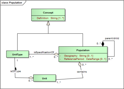
Figure 8: Population
[Source: GSIM v1.1 Enterprise Architect file]
For the RIM, we will only need to extend this model to better describe the relations between Units, as these are not part of this model in GSIM. The proposal we saw above was to have an explicit Relationship information object between Units. The Relationship information object and its relationships to Units would be extensions of the GSIM model. They would be typed "hasRelationshipWith" or "hasRelationshipTo". The Relationship object itself is also typed, describing what the relationship is – this would be a property (ie, "employedBy", "marriedTo", etc.). See earlier discussion of relationships in the Datum-Based Data Structure section 4.3.

8.3 Variables

As we have seen, there are three types of variables in GSIM, which will all be useful in the RIM.

Figure 9: Variable and Represented Variable
[Source: GSIM v1.1 Enterprise Architect file]
Here, we see how Variables (relating to a Conceptual Domain) are sub-classed from Concepts and Represented Variables take their meaning from Variables, but have Value Domains corresponding to the Variable's Conceptual Domain. An Enumerated Value Domain is represented by a Code List information object, which could be based on a Statistical Classification (see the next section).
Instance Variables are shown in the diagram below:

Figure 10: Instance Variable
[Source: GSIM v1.1 Enterprise Architect file]
Here, we see how an Instance Variable takes its meaning from a Represented Variable, which specifies the value it may hold as a Data Point (taken from the Value Domain of the Represented Variable). We can also see how an Instance Variable measures a Population, whose members are specified by a Unit Type. What we do not find in this diagram is that each Instance Variable would contain a value pertinent to a specific Unit coming from within that Population. This is implicit in GSIM, as you could have Populations made up of individual Units – in the RIM, we make this explicit. Further, we see how Instance Variables hold the specific values used in describing data corresponding to our Data Structure Components (Identifier Components, Measure Components, and Attribute Components).
For the RIM, we will use all of these types of variables. Represented Variables will be reused across the time-specific views in our Analysis Data Sets (ie, the employment status variable is a Represented Variable, which will have an Instance Variable for a specific individual Unit across each observational period in the Analysis Data Set). The Variable itself is useful when two Represented Variables have different representations, and need to be re-coded, etc. They share the same Concept, but have different representations over time, which can be aligned only through processing.
For RIM, one or more attributes will need to be added to the GSIM Variable information objects to support disclosure control. Examples of these could be discoverability, sensitivity, etc. Represented Variable is extended to add a sensitivity attribute.

Figure 11: RIM Represented Variable extension

8.4 Value Domains, Statistical Classifications, and Codelists

As visible in the diagrams above for Variables, we have an association between the Represented Variable and the definition of its representation (the Value Domain object). There are two distinct cases – all described by GSIM – in the RIM:

1. Described Value Domains
2. Enumerated Value Domains, Code Lists and Statistical Classifications

The first case is the simplest: the Described Value Domain describes a typed value (a string, a specific numeric type, a time and/or date value, etc.) These are not enumerated, but are structured according to some known system describing their allowed values.
The information objects in the second case are closely related, because what is actually implemented is a Code List information object (in GSIM terms). In GSIM, Code Lists, Statistical Classifications and Category Sets share a common basic structure, which allows them to be implemented almost identically, as seen in the diagram below.
The key object in GSIM is the Node Set, which provides the basic structure for Statistical Classifications, Category Sets and Code Lists. Although there is a large amount of detail in GSIM regarding Statistical Classifications, this level of detail is not needed for all information objects in RIM. For the values of enumerated Represented Variables, we will need to know the Code List and each of the Code Items which make it up. The Code Items are Nodes, linking a Category (a meaning) with its Designation (the code itself). This same structure is seen for Statistical Classifications and Classification Items, with the difference that Statistical Classifications can have hierarchical relationships among their Classification Items. This is important in the RIM for handling disclosure control (it is possible to aggregate up on the hierarchies within a Statistical Classification). Further, it is necessary to understand the Level information objects, which correspond to the hierarchies within Statistical Classifications. These allow for the understanding of how individual Classification Items correspond to real-world constructs. A good example here is geography – the Levels could describe Countries, Counties, Municipalities, etc.

Figure 12: Node
[Source: GSIM v1.1 Enterprise Architect file]
Further, the RIM will use the Map construct from GSIM, in cases where two Represented Variables have Nodes which correspond, but are not identical. Maps are organized into Correspondence Tables, and can show where two Nodes (whether from Code Lists, Category Sets or Statistical Classifications) are equivalent.

Disclosure Control Rules and Risk Minimization Actions

This section presents the information model to support the application of disclosure control and risk minimization in RAIRD. Disclosure control operates on the Provisional Output, before a Final Output can be shown to the researcher. This model makes no attempt to venture into the domain of methodology in this area. It is based on the assumption that a useful methodology can be expressed as a series of Rules, operating on the data and metadata available for the Provisional Output.

9.1 GSIM and Disclosure Control

GSIM views disclosure control as it does any other statistical process – it is a Business Process which is implemented via a Business Service, Process Steps and related information objects. The application of the GSIM model for this process in RAIRD is presented in the Process Descriptions in section 10.
For the RIM, a specific model of the information objects required to support this process is needed at a level of detail which goes beyond what GSIM offers us.
There are two relevant information objects in GSIM: Rules and Process Methods. These objects are found in the Process Design portion of GSIM (GSIM Specification v1.1 Figure 4). The Process Method has a set of Rules through which it will be implemented when the process is executed. The RIM model builds on these objects, but adds more specificity to the model.
The RAIRD process involves more than just the application of Rules – it also associates Corrective Actions with the Rules. In order to be meaningful, these Corrective Actions must operate on identified parts of the data being checked.

9.2 RIM Model

The diagrams below show the RIM model for disclosure control information objects. Some of these objects are extensions of GSIM information objects: Disclosure Control Rules are extensions of GSIM Rules; Disclosive Data Point and Non-Disclosive Data Point are extensions of GSIM Data Point; and the Provisional Output and Final Output are extensions of GSIM Data Set.
In the first diagram, we see the identification of potentially disclosive data:

Figure 13: Disclosure Risk Assessment
Here, the application of a Disclosure Control Rule to a Provisional Output produces a Disclosure Risk Assessment by identifying Disclosive Data Points and Disclosive Data Point Combinations. The Provisional Output has Non-Disclosive Data Points, Disclosive Data Points, and Disclosive Data Point Combinations. The Disclosive Data Point Combinations may be composed of Disclosive and/or Non-Disclosive Data Points.
There is the possibility of an up-front Disclosure Risk Assessment, in which some attributes may be assigned to variables (i.e. discoverability, sensitivity) while other aspects of Disclosure Risk Assessment can only be known at the time of disclosure control (e.g. granularity, skewness), because they depend on understanding the context within which a variable is being used, and on having Disclosure Control Rules which guide the Disclosure Risk Assessment.
The second diagram shows the information objects and their relationships after the potentially disclosive data has been identified:

Figure 14: Disclosure - Corrective Actions
The Disclosure Control Rule identifies one or more Corrective Actions which are informed by the Disclosure Risk Assessment. The Provisional Output is transformed by the Corrective Actions, through operations on Disclosive and/or Non-Disclosive Data Points. (These operations could be aggregations made in reference to the classifications associated with the Data Points; they could be cell suppressions, or the application of any other formal techniques.) The result is a Final Output deemed to be at an acceptable distribution risk level. As Corrective Actions are applied, it is possible that interactions with the researcher occur, so that the Final Output is maximally useful for their purposes.

Process Descriptions

This section attempts to describe the processes specific to RAIRD using the GSIM version 1.1 model. There are several areas in which the processes to be used by RAIRD are fairly specific, notably the processing and transformation of data, and the execution of tabulations, regressions, and similar analysis functions. These are not covered in this document. The RAIRD-specific functions – including accreditation of organizations and researchers – are included. We will provide extensions to the GSIM model for the RIM because these are areas which are not covered in GSIM.
The GSIM Process model is very generic, and allows for many different types of processes to be described. However, it is a model designed to describe statistical processes, and such processes as organizational accreditation do not fall within this category. Thus, there is a difference between these two sections of this document.
GSIM 1.1 offers a great deal of detail about Process Design, much of which is potentially relevant to the RAIRD. This document describes both the design-time and run-time parts of the GSIM Process descriptions.
The processes covered here include the Load the Event History Data Store Process, the Interact with the Virtual Research Environment Process, and the Control Disclosure Risk Process, using the GSIM run-time Process model. The Accredit Institution Process and Manage Users Process are described, but not using the GSIM information objects intended only to describe statistical processes.

10.1 The GSIM Process Model

Below are the parts of the GSIM model which will be most important for describing RAIRD processes. Note that this model can be used at different levels: RAIRD could be described as a single process using GSIM, with several sub-processes. That is interesting from the perspective of a statistics organization using GSIM to manage its production lifecycle, where RAIRD itself could become a dissemination service. For the purposes of describing and supporting the implementation of RAIRD, however – the goal of the RIM – this very high-level view is less useful. Instead, we will look at a level of detail which is slightly greater.
There are two diagrams in GSIM which are of greatest interest: the design-time process model, and the run-time process model. Note that in GSIM, a process can be automated, manual, or a combination of the two – all kinds of process execution are modeled in the same way.
The design-time model for processes has already been mentioned, as it contains the Rule and Process Method information objects which are used in the RIM for modeling information used in disclosure risk control. This diagram is shown below:

Figure 15: Design Processes
[Source: GSIM Specification v1.1 Figure 4]
The entire RAIRD project plan and related materials could be seen as a Statistical Program Design in this diagram – it specifies the Business Functions to be supported, and ultimately creates the Process Designs through which this will be achieved. Note that GSIM Process Designs may utilize Process Designs for sub-processes. Because there is often conditional logic in the way that sub-processes are executed, this logic must be specified. This is the Process Control Design. Another important aspect of the Process Design is the specification of what types of inputs and outputs the Process has. We find these in the Process Input Specification and Process Output Specification information objects. The Process Design itself is informed by some Process Methods, which are the basis for the formulation of Rules which drive the Process Control Design of the process.
Here is the GSIM diagram describing the running of processes:

Figure 16: Run Process
[Source: GSIM Specification v1.1 Figure 6]
In each case, we have a Business Process – the overall goal, described not in technical terms, but in terms of the business goal. A Business Process can execute a Process Step, or execute a re-useable Business Service. The latter information object is more appropriate here, because RAIRD has the goal of implementing re-useable functionality. Business Services execute Process Steps, just indirectly.
All Process Steps are specified by a Process Design – this is the work needed to determine exactly how a Process Step will be executed, and this typically exists in some documentary format. A Process Control is the flow logic associated with a Process Step, among its sub-Process Steps. The Process Control corresponds to its Process Control Design.
When executed, specific Process Inputs are specified, as well as specific Process Outputs. These must agree with the types of inputs and outputs specified in the design phase. The information about the process execution itself (logs, etc.) is seen in the Process Step Instance, which holds all the information about the execution (e.g. success, failure, error).

10.2 Load Event History Data Store Process

In this process, we have the Business Process of taking the needed data and metadata and loading it into the Event History Data Store. This overall process is executed as a Business Service, which is implemented as an API (Application Program Interface) taking specified inputs (see below). Load Event History Data Store process uses a top level Process Step –– which in turn has several sub-Process Steps:
The overall Process Step is composed of several sub-Process Steps:

1. Validate
2. Transform
3. Load

Each sub-Process Step is described below.
Process Control:
If the information is validated successfully, it passes to the preparation/transformation stage (sub-Process Step). Once prepared/transformed, it is passed to the load stage.
Normal logging will be performed to populate the Process Step Instance.
Sub-Process Step 1: Validate
This sub-Process Step takes the Event History Input Data Set and the Input Metadata Set and validates that the data is completely and validly described according to its structure. This includes checking not only the event history file(s) against its immediate structural description, but also checking that any references external to the data file(s) (references to variables described in the base metadata package, and any Statistical Classifications/Codelists used by these) are correct. Outputs include an indication of success or failure, and any error messages needed to correct fatal errors for load, or warnings to spot possible errors which should be investigated by a staff member.
Sub-Process Step 2: Transform
This sub-Process Step performs any needed calculations/transformations on the input data, using whatever metadata is needed, so that the Event History Data Store can be populated with any additional information which can be derived from that supplied, including search indexes, calculated values, etc.
Sub-Process Step 3: Load
This process takes all prepared information and loads it into the Event History Data Store. Outputs include an indication of success or failure and any errors or warnings generated by the load process.

10.3 Interact with the Virtual Research Environment Process

This process serves the purpose of allowing researchers to become familiar with the contents of the Event History Data Store, to create Analysis Data Sets, and to explore, process and analyze the data to create Provisional Outputs. The functionality is executed by several of GSIM Business Services: those offered for browsing the Data Catalogue, and for executing various operations on the data through the Virtual Statistical Machine.
The overall Process Step is composed of several sub-Process Steps:

1. Browse the Data Catalogue
2. Select Variables for the Analysis Data Set
3. Process Analysis Data Set
4. Create Provisional Outputs

Each sub-Process Step is described below.
Process Control:
Each of the sub-Process Steps may be performed in any order, and repeated as often as needed. The primary interactions are determined by the researcher, who acts as the decision-maker in determining which sub-Process Step to execute next. The process execution is done when a Provisional Output is submitted for finalization. At this point another process is invoked: Control Disclosure Risk Process.
Sub-Process Step 1: Browse the Data Catalogue
This sub-process allows access to the metadata contained within the Event History Data Store, through the VRE browser interface. The Process Inputs to this process are the metadata themselves, which are largely based on the Input Metadata Set, but enhanced with additional information calculated during the load process, and including presentational content. (Note that in GSIM terms, the presentational content is a Presentation object, and the Data Catalogue is a Product.)
There are no Process Outputs, since the goal of the sub-process is to inform the researcher about the data available in the Event History Data Store.
Sub-Process Control 1:
The researcher drives this process by navigating through the metadata. This may involve searches on keywords, viewing according to topical structure (all functionality based on Concept Systems), and exploring Units and Represented Variables. There is also additional information about which data are available for which time periods, and how they are associated with Units.
Sub-Process 2: Select Variables for the Analysis Data Set
This process allows the researcher to create or add variables to the Analysis Data Set by requesting variables one at a time, and either specifying a point in time (for static variables) or a time period (for event history variables). When selecting variables, the observation periodicity may need to be specified. The researcher may continue to add data to an existing Analysis Data Set, or may clear the existing one and start to create a new one.
The inputs to this process are the Datum-Based Data Set held in the Event History Data Store, and the outputs are Analysis Data Sets.
Every operation in this sub-process is logged, and is available to the researcher, so that Analysis Data Sets may be accessed at any stage of their evolution. This allows researchers to come back to any iteration of any Analysis Data Set, even after having invoked another sub-process within the overall process.
Sub-Process Control 2:
The researcher drives this process by making selections through the browser-based VRE. Because every iteration of every Analysis Data Set is available to the researcher at any point during the overall process, even after executing other sub-processes, the flow of this sub-process is very flexible.
Sub-Process Step 3: Process Analysis Data Set
This process allows the researcher to manipulate the Analysis Data Set in ways that do not involve the addition of variables from the Event History Data Store. Several operations are possible, such as collapsing the data set to aggregate some variables, reshaping the data (transposing rows and columns), recoding variables, generating new variables by performing computations on existing ones, etc. The Business Service being invoked is the Virtual Statistical Engine.
As these operations are performed, they are logged, and the iterations of the Analysis Data Set are accessible to the researcher, so that it is possible to re-create the Analysis Data Set at any point, even after invoking other sub-process steps in the overall process.
The Process Inputs to this sub-process are the Analysis Data Set, and the Process Outputs are modified Analysis Data Sets and the log of what operations have been performed.
Sub-Process Control 3:
The researcher drives this process by executing processing operations through the browser-based VRE. Because every operation made on any Analysis Data Set is available to the researcher at any point during the overall process, even after executing other sub-processes, the flow of this sub-process is very flexible.
Sub-Process 4: Create Provisional Outputs
This sub-process allows researchers to perform analytical operations on the Analysis Data Set to produce Provisional Outputs, which may then be submitted for finalization. These operations include the running of tabulations, regressions, correlations, and similar analytical functions. The Business Service being invoked is the Virtual Statistical Engine. As for other user operations in the VRE, analytical operations are logged and made available to the researcher, so that all iterations of the Provisional Outputs may be retrieved at any time, including those which were not submitted for finalization.
The Process Inputs to this sub-process are the Analysis Data Set, and the Process Outputs are Provisional Outputs.
Sub-Process Control 4:
This sub-process has the potential for ending an iteration of the overall process if the researcher requests that a Provisional Output be finalized, to produce a Final Output. A request for finalization always invokes the execution of the Control Disclosure Risk Process. If the researcher does not attempt to finalize a Provisional Output, then this sub-Process may be combined with the other sub-Processes as flexibly as the others.

10.4 Control of Disclosure Risk Process

This process performs the Business Purpose of checking requested outputs of the analysis process against a set of rules designed to minimize risk of disclosure. The Business Service is the Disclosure Control System, and the inputs are the Provisional Output, relevant metadata describing the Provisional Output (including classifications to be used for aggregation), the set of Disclosure Control Rules for checking the Provisional Output against, the Disclosure Risk Assessment, and the set of Corrective Actions to be taken in case of failure. The output is an acceptable Final Output.
The overall Process Step is composed of several sub-Process Steps:

1. Apply Rules and Identify Risk
2. Negotiate Corrective Actions
3. Correct the Provisional Output

Each sub-Process Step is described below.
Process Control:
If the first sub-Process Step fails, then the second sub-Process Step is invoked. Otherwise, no transformation is required and the Provisional Output becomes the Final Output because it is already safe. It is possible that the first two sub-Process Steps will iterate several times until an acceptable Final Output has been created.
Sub-Process Step 1: Apply Rules and Identify Risk
The Disclosure Control Rules are applied to the Provisional Output, and if any of the checks fail, the points of failure within the data are identified. The inputs to this sub-Process Step are the Disclosure Control Rules, any Disclosure Risk Assessments, and the Provisional Output. The outputs from this step are an indicator of success or failure, along with details about which checks failed and what the points of failure are within the Provisional Output, as well as a modified Disclosure Risk Assessment. If the Disclosure Risk Assessment deems the Provisional Output acceptable, then this is promoted to being a Final Output, and shown to the researcher.
Sub-Process Step 2: Negotiate Corrective Actions
The results of the preceding sub-Process Step are presented to the user for input regarding priorities for possible Corrective Actions. The resulting output is passed to the next sub-Process Step.
Sub-Process Step 3: Correct the Provisional Output
In the case that there have been failures in checking the Provisional Output against the Disclosure Control Rules, transformations will be performed to create an acceptable Final Output (eg, cell suppression, aggregation, etc.) Inputs are the outputs of the preceding sub-Process Step, plus the Disclosure Risk Assessment, and the Corrective Actions. The output is the Final Output to be passed to the researcher.
All information about rules, actions, input and output tables, etc. are logged along with user details for re-use and audit-trail purposes.

10.5 Accredit Institutions and Manage Users Process

As mentioned in the Introduction, this process is not modeled using GSIM because it is not a statistical production process. Viewing it as a set of inputs and outputs to a transformative process is not particularly useful. Despite this, it is important to have some information objects in the RIM which will cover the needed information.
There are two aspects to this process, which are separated in time. Before any researcher can gain access to RAIRD, the institution with which they are affiliated must become accredited. Accreditation is performed by the agency which operates RAIRD and maintains the event-history data. Once accredited, researchers may request access to RAIRD, at which point they become managed users who can be given access to the system. Note that this process does not describe run-time user authentication, as that is a generic process which presumably exists within the IT infrastructure of any organization. Rather, this process is simply the creation of the information to be managed so that run-time authentication and other needed generic processes can be performed. This process can be seen in the following diagram:

Figure 17: Accredit Institutions and Manage Users Process Flow
Here, we see the overall process of exchange. This diagram does not show all of the information objects needed to support the process, but indicates the activities which are taking place.
The Research Institution wishing to be accredited makes an Accreditation Request to the Accrediting Organization (the statistical agency operating RAIRD), which will either be approved or denied. If the Accreditation Request is denied, then a Refusal Rationale is provided, which may form the basis for further Accreditation Requests. If the Accreditation Request is approved, then the Accrediting Organization will record the accreditation, and provide the Access Agreement to the requester for acceptance.
Once accredited, users and projects wishing to access the RAIRD will send Access Requests to the Accrediting Organization, which – if approved – will result in the setting up of User and Project Profiles, provision of username and password, project start- and end-dates, and other needed information.
If the Access Request is denied, then a Refusal Rationale will be provided so that a more appropriate Access Request can be re-submitted, if desired.
The following diagram shows the information objects involved in the Accredit Institutions part of this process:

Figure 18: Accreditation
In this diagram, we can see that there will be information about the Research Institution submitting the Accreditation Request (it is assumed that the Accrediting Organization is operating RAIRD, and therefore we do not model the internal records a statistical agency maintains about its own operations.) The Research Institution will be linked to the Accreditation Request, and this request will further be related either to an Access Agreement, a Refusal Rationale, or both (if accreditation is granted after one or more earlier refusals).
The part of the process concerned with Access Requests has a set of information objects, building on the information objects we see in the accreditation-related part of the model:

Figure 19: Researcher Access Request
We still have the information objects representing the Research Institution and the Access Agreement, but these are now placed in the context of the actual Access Request from a research Project.
The Project is an information object with several properties, among which are the start and end-dates granted for data access. These result in an Access Request, submitted by the Project (which may be as small as a single Researcher). Access will be granted based on the accreditation status of the Research Institution, plus a review of the Researchers (eg, training certificates). If refused, a Refusal Rationale would be associated with the Access Request so that it could be corrected and re-submitted.
There are two types of Researchers – primary Researchers, who have special legal responsibility for the Project, and other Researchers. Some of the properties for Researchers are their degree status, training certification, and contact details. The User Profile is the information which RAIRD manages about users who are allowed access to the system: username and password, information about different activities for re-use and audit trail, saved data of any sort, preferences, etc. Similarly Projects have their own Project Profiles, as there is a set of similar information for data shared among all Researchers who are part of a Project.
The output of a Project is ultimately a Research Publication (this may be done by an individual Researcher or by the Project as a whole). Tracking the Research Publications for which RAIRD data was used is a requirement for the purposes of auditing should any prove disclosive in the future.
It should be noted that there will be several different levels of users for the overall system, and this will be a factor in controlling disclosure risk, as some levels of users are deemed riskier than others. Depending on the level of the users, the disclosure control would be more or less restrictive in terms of what Provisional Outputs could be finalized.
Users may be classified in 4 categories based on data needs and institutional infrastructure:

1. Standard users: National and international institutions needing large quantities of data for single projects.
2. Specific, large users: National and international institutions with continuous projects and/or many projects which are topically related and which often request long time series.
3. Institutions with special requirements concerning health registers.
4. Students.

i)    Standard users

This category contains the majority of potential users. It is a very diverse group, but often with a need for updates of data. It is expected that a remote access solution will function well for this user category, in particular because of lessened bureaucracy.

ii)   Specific, large users

This group is smaller in numbers, but contains more sophisticated large-scale data users. In particular it represents more long-term projects that also include substantial amounts of added value to their research data. This category of users is not as easy to satisfy through a remote access solution. An investigation into possibilities for offering more automated services also to this group of users is planned as part of the application.

iii)  Institutions with special requirements within health registers

Within the health register system there are some specific regulations that have led to a specific mode of operation for merging of data. Only the researcher is allowed to keep the merged data. The present procedure is difficult to automate, but an investigation into possibilities for procedures giving more efficiency and security is planned, based on experiences built up from other areas.

iv)  Students

Education is in need of data that facilitates more relevant work and training. Such data are generally easier to standardise, aggregate or anonymize. A secure data system is the most relevant solution here.

References

The following sources of information have been used:
RAIRD: http://www.raird.no
GSIM: http://www1.unece.org/stat/platform/display/gsim/Generic+Statistical+Information+Model
Particularly Specification v1.0 incl. Annex C: Glossary and Annex D UML class diagrams and object descriptions, but also GSIM v0.8 Annex D Expanded Set of Principles.
GSBPM: http://www1.unece.org/stat/platform/display/GSBPM/Generic+Statistical+Business+Process+Model
DDI Specification: http://www.ddialliance.org/Specification/
ELSST: http://elsst.esds.ac.uk/Home.aspx

1. See: www.raird.no ↩
2. (If DDI Lifecycle is used, there would be two "types" of metadata being loaded: the structural description and the "study-unit"-specific metadata (a direct description of the data being loaded); and the underlying foundational metadata, giving such things as the list of variables in the register data, the representations and classifications of variables, their labels, any associated concepts, their unit types and relationships, etc. This latter set could be transmitted using a DDI "resource package".) ↩
3. Each of the many records documents a single datum, in a record structure which would contain an ID, a reference to the value's variable, the value itself, and start- and end-dates for the event measured by the variable (or period of the observation [eg, for yearly data, year = 2005], in the case of a snapshot of the data). The variable reference points to a variable documented in the metadata package (part of the Input Metadata Set) loaded at the same time. When loaded into the store, the classifications used by different variables would be stored each in their own tables, like a traditional star-schema based data warehouse. Other associated metadata such as labels could be attached in a similar fashion. More documentary information could be held in the database at whatever level of granularity is desired. ↩