UNECE – HLG-MOS Machine Learning Project

Classification and Coding Theme Report

PDF version

Author: Claus Sthamer (Office for National Statistics, UK)

* Visit WP1 Pilot Study Wiki Page for reports of the pilot studies conducted under Coding and Classification Theme

Table of Contents 

1. Background

2. Overview of Classification and Coding

3. Data pre-processing

4. Algorithms

5. Quality measure used in Classification and Coding

6. Classification and Coding Pilot Studies

7. Value added by Classification and Coding using ML in the production of official statistics

8. Expected value added not shown 

9. Best practises

10. Comparison of results

11. Conclusions

1. Background

The UNECE Machine Learning project was recommended by the HLG-MOS – Blue Sky Thinking network in the autumn of 2018, approved early 2019 and launched in March 2019. The objective of the project is to advance the research, development and application of Machine Learning (ML) techniques to add value to the production of official statistics. ¹ Three themes were investigated:

• Classification and Coding
• Editing and Imputation
• Imagery

This report attempts to summarise and investigates how and if the pilot studies carried out on Classification and Coding have shown to make official statistics better, where better can be any one or more aspects of:

• Cheaper
• Faster data release
• More consistent data
• Alternative data sources

Advances made to their respective organisation will also be investigated.

This report will also show a broad range of approaches and ML algorithms tested and used and the different results associated with that. This richness is a testament of the commitment and contribution of all the NSO (National Statistics Offices) involved and their commitment to this project.

2. Overview of Classification and Coding

“Classification is the problem of identifying to which of a set of categories (sub-populations) a new observation belongs, on the basis of a training set of data containing observations (or instances) whose category membership is known. Examples are assigning a given email to the "spam" or "non-spam" class, and assigning a diagnosis to a given patient based on observed characteristics of the patient (sex, blood pressure, presence or absence of certain symptoms, etc.). Classification is an example of pattern recognition.

In the terminology of machine learning, classification is considered an instance of supervised learning, i.e., learning where a training set of correctly identified observations is available. The  corresponding unsupervised procedure is known as clustering, and involves grouping data into categories based on some measure of inherent similarity or distance.” ² As far as this theme report is concerned, the given set of data referred to in the above quote is typically a text or narrative provided by the respondent to describe, for example, their occupation, the industrial activity of a company, injury information of an injured worker, product descriptions scraped from the internet or sentiment text obtained from Twitter. Most of the pilot studies fall into the group of Multi-Class ³  classification tasks. These aim to classify text descriptions into internationally accepted coding frames, e.g. SIC, SOC, NAICS, NOC or ECOICOP that offer many target classes, see Table 1 for a list of the coding frames used in the pilot studies. Even though the aim of these studies appears to be mostly the same, their approach and software solutions used differ as their results do too.

Table 1 – Coding Frames

There was only one pilot study with binary classification, the twitter sentiment classification into positive and negative sentiments. The target classes for this are [‘Positive’, ‘Negative’].

For example:

“The UK Standard Occupational Classification (SOC) system is used to classify workers by their occupations. Jobs are classified by their skill level and content. The UK introduced this classification system in 1990 (SOC90); it was revised in 2000 (SOC2000) and again in 2010 (SOC2010).” ⁴ Table -2 Some entries from the SOC-2010 coding frame: ⁵

In Table 2 are some entries from the SOC coding frame shown. A SOC code classification task has to assign a code from the table to the textual narrative given by the respondence. That narrative could be: “I drive a fork-lift truck” or “I use fork-lift trucks in my job to load up lorries”

The natural language narrative, the survey variable or feature, has to be assigned to the correct code or class.

The term feature is here used synonymous with the term ‘independent variable’, both are often used in Machine Learning terminology. Features in the data set are for example: Age, Job Description, NetPay or Description of Injury.  Feature selection is then the process of selecting the best subset of relevant input features to be used by the Machine Learning algorithm to build a model. These features can also be called Predictor features as they are used by the model to build its internal rules and structure to predict one or possibly a number of target features.  The predictive ability of the ML algorithm can sometimes be improved with feature engineering. This is done by transforming raw data into new features that better represent the underlying problem to the ML algorithm.

3. Data pre-processing

Data pre-processing is needed to some degree by all Machine Learning algorithms. For Natural Language Processing (NLP), some techniques can be used to remove bits from the text that at their best do not add information and at their worst produce noise in the data and reduce the ability of the ML algorithm to recognise words of the same meaning.

Most pilot studies have done a lot of work in this area and have shown that these techniques can have an influence on the predictive ability of the ML solution.

Removal of stop-words: Stop words are words like “the”, “a”, “an”, “in”. These are unimportant words in natural Language Processing (NLP), they do not add much meaning to the text to be analysed. By removing these words, the algorithm can focus in the important words.

Stemming and Lemmatisation are two approaches to handle inflections, the syntactic difference between word forms. Both Stemming and lemmatisation can be achieved with commercial or open source tools and libraries.

Stemming: This is a process where words are reduced to their stem or root by chopping off the end of the word in the hope to reduce it to its stem, e.g. the word “flying” has the suffix “ing”. The stem is “fly”.

This is typically done with an algorithm. The aim is to reduce the inflectional forms of each word into a common base. This increases the occurrence of the word and gives the algorithm more to learn on. The Porter Stemmer algorithm is very popular for the English language, it chops both “apple” and “apples” down to “appl”. This shows that stemming might produce something that is not a real word. But if this is done to all the narratives to be classified and all target documents, the algorithm can find matches.

Lemmatisation: This also tries to remove inflections, but it does not simply chop off these inflections. It uses lookup tables, e.g. WordNet, that contain all inflected forms of the word to find the base or dictionary form of the word, which is known as the lemma, e.g. “geese” is lemmatized by Wordnet to “goose”

If the word is not included in the table it is passed as the lemma.

Normalisation to lower case: Every word is converted to lower case.

n-gram: The text to be classified is chopped up into words or character sequences. To chop them up into syllabus is much harder as these depend on enunciation and are harder to calculate.

For the narrative “the fox jumps over the fence”

• word 1-gram: the, fox, jumps, over, the, fence
• word 2-gram: the fox, fox jumps, jumps over, over the, the fence
• character 3-gram: ‘the’, ‘he_’, e_f’, ‘_fo’, ‘fox’, ‘ox_’, ‘x_j’, ‘_ju’ ……..

For the space character the underline ‘_’ is used here.

The Mexican pilot study on occupation and economic activity classification describes in great detail their work on n-grams and what impact changes in the n-grams have on their prediction results.

However, the U.S. Bureau of Labour Statistics (BLS) stopped using stop-word removal or stemming after they found out in early experiments that these techniques proved to be unhelpful due to the nature of the text narratives they need to classify. But they used CountVectorizer as a tool to create a “bag of features” representing the input. It shows which words (or sequences of words, or sequences of characters) occur in the input, but not the order in which those words or sequences appear. When they moved over to Neural Networks, they stopped this too. Preserving the original ordering of the sequence of letters allows the Neural Network to gain more insight into the text while simpler algorithms are not capable of learning the intermediate representations, i.e. that letters form words, and words form phrases and sentences, and sentences form paragraphs and so on.

Please see the column Data Pre-processing in Table 4 for steps carried out by all the pilot studies.

4. Algorithms

Here is a brief overview of the various ML algorithms used by the Classification & Coding pilot studies.

4.1 Random Forest

The Random Forest algorithm, like its name implies, creates a large number of individual decision trees that operate as an ensemble. Each individual tree in the random forest spits out a class prediction score and the class with the most votes becomes our model’s prediction. ⁶ For each class, a score is given for the data to belong to that class. Let us assume we have a classification task to classify animals into 4 classes (cat, dog, mouse, fish), these 4 classes are the target for the data.

Training of this machine learning algorithm is done with labelled cases, that are data records, in this case with details about animals, but each record as already been assigned to which class it belongs. The Random Forest algorithm is initialised with a set of hyperparameters that control the behaviour of the algorithm. One of them is the number of trees it builds for the prediction task, e.g. n_estimators = 1000 instruct the algorithm to build 1000 trees out of a random selection of data set features and data records.

When the learned model is used to predict into which class a record falls, a score is given for each class, e.g. [0.15, 0.30, 0.45, 0.10]. In this case the highest score is 0.45, meaning that 450 out of the 1000 trees voted for the 3^rd class which is ‘mouse’ in our example. The Random Forest Machine learning model predicts that ‘mouse’ is the most likely classification of this record.

Random forest is a flexible, easy to use machine learning algorithm that produces, even without hyper-parameter tuning, a great result most of the time. It is also one of the most used algorithms, because of its simplicity and diversity (it can be used for both classification and regression tasks). ⁷ This algorithm was used in 6 of the pilot studies and in some cases, it has outperformed any other algorithm in their experiments and uses relatively little computer resources just like Logistic Regression (see 4.2) and SVM (see 4.3)

4.2 Logistic Regression

Contrary to Linear Regression which predicts a continuous value, e.g. age or price, Logistic Regression can be used to predict a categorical variable from a given set of independent variables. It is used to predict into which discrete values (0/1, yes/no, true/false) a data record falls and it does this by fitting the data to a logarithmic or logit function. For this reason, the algorithm is also called logit regression. ⁸  Logistic Regression has been used in 7 of the pilot studies.

4.3 Nearest Neighbour (k-NN)

The k-NN algorithm treats the features as coordinates in a multidimensional feature space and then places unlabelled data into the same category or classes as similar labelled data or Nearest Neighbours (NN).

For a given data record it locates a specified number K of records in the training data set that are the “nearest” in similarity. The classes these neighbours belong to are counted and the case is assigned the class representing the majority of the k nearest neighbours.

If there are more than two possible classes this classifier has to pick from, it will pick the most common class represented by the k neighbours. This algorithm is also called k-NN. It is known as a “lazy“ machine learning algorithm as it does not produce a model, its understanding about the relationships of the features to a class is limited. It simply stores the training data and then calculates the Euclidean distance between the new record to the training data and then picks the k nearest to label the new record.

4.4 SVM

With the Support Vector Machine (SVM) algorithm significant results can be achieved with relatively little computing power. In this classification algorithm each data item is a point in a n-dimensional feature space where n is the number of the features or variables of the data set used. If we only have two features, the SVM algorithm finds a line that is the maximum distance away from the nearest point of each class to this line. For many features a hyperplane is found that separates best the labelled data points belonging to each class, this is called the Maximum Margin Hyperplane (MMH)

The points from each class that are the closest to the MMH are called Support Vectors (SV). Each class must have at least one, but may have more than one SVs. These SV define MMH and thus provide a very compact way to store a classification model.

To predict which class a new data record belongs to, that data point is drawn and the class area it falls into is the predicted class. In this way, SVM learning combines aspects of both the instance based Nearest Neighbour and regression methods. As this combination is very powerful, SVMs can model highly complex data relationships which accounts for the good results achieved with this classifier in 5 pilot studies.

4.5 FastText

FastText was created by Facebook’s Artificial Intelligent (AI) lab. It is a library for efficient learning of word representations and sentence classification. The model allows to create an unsupervised learning or supervised learning algorithm for obtaining vector representations for words. Facebook makes available pretrained models for 294 languages. FastText uses a neural network for word embedding. ⁹

4.6 Naïve Bayes

It is a classification technique based on Bayes’ Theorem with an assumption of independence among predictors. In simple terms, a Naive Bayes classifier assumes that the presence of a particular feature in a class is unrelated to the presence of any other feature. For example, a fruit may be considered to be an apple if it is red, round, and about 3 inches in diameter. Even if these features depend on each other or upon the existence of the other features, all of these properties independently contribute to the probability that this fruit is an apple and that is why it is known as ‘Naive’.

The Naive Bayes model is easy to build and particularly useful for very large data sets. Along with simplicity, Naive Bayes is known to outperform even highly sophisticated classification methods. This algorithm is mostly used in text classification and with problems having multiple classes. ¹⁰ It is also the computational cheapest algorithm. This algorithm was used in 4 pilot studies.

4.7 Neural Networks

Neural Networks have been used in two pilot studies for text classification:

• Mexico for the classification of occupation and Economic activity.
• USA – BLS for the classification of workplace injuries use Multi-Layer Perceptrons, Convolutional and Recurrent Neural networks.

These algorithms require expensive and powerful hardware as shown by these two pilot study reports. But they are also very powerful in ‘learning’ patterns in the data that relate to the target, in these cases to complex coding frames.

The work done by BLS has shown that extensive pre-processing typically carried out for other ML algorithms is not needed, or can even be detrimental when neural networks are used because information from the text is lost for the learning process.

4.7.1 Multi-Layer Perceptrons

A Multi-Layer Perceptron (MLP) is a type of feedforward Artificial Neural Network (ANN). It consists of input nodes that receive signals, nodes in one or more hidden layers and one or more output nodes. Signals travel from the input, via the hidden layers to the output. Each input node is responsible to process a single feature of the data set. The value of this feature is then transformed by the activation function of this node. The result of this is then passed onto each node, but weighted, in the next layer. The more complex the MLP, the more complex relationships in the data can be recognised. The processing expense grows rapidly with the number of layers and neurons in each layer. Not even the 100000 neurons of a fruit fly can yet be simulated with a ANN.

4.7.2 Convolutional Neural Networks (CNN) and Recurrent Neural Networks (RNN)

Convolutional and recurrent neural networks are types of neural networks designed to efficiently learn specific relationships in the data. Convolutional neural networks were originally designed for image processing and focus on efficiently learning spatial patterns.

In Recurrent neural networks, signals are allowed to travel backwards using loops. This ability mimics more closely how a biological neural network operates. This allows extremely complex patterns to be learned. The addition of a short-term memory or delay increases the power of RNNs, this includes the ability to learn sequential patterns. Both approaches have been found to be useful for a variety of language processing tasks and are therefore powerful classification tools.

4.8 XGBoost

XGBoost stands for eXtreme Gradient Boosting. The XGBoost library implements the gradient boosting decision tree algorithm and is one of the fastest implementations for gradient boosting. This algorithm goes by lots of different names such as gradient boosting, multiple additive regression trees, stochastic gradient boosting or gradient boosting machines. Boosting is an ensemble technique where new models are added to correct the errors made by existing models. Models are added sequentially until no further improvements can be made. A popular example is the AdaBoost algorithm that weights data points that are hard to predict.

Gradient boosting is an approach where new models are created that predict the residuals or errors of prior models and then added together to make the final prediction. It is called gradient boosting because it uses a gradient descent algorithm to minimize the loss when adding new models. This approach supports both regression and classification predictive modelling problems. ¹¹

5. Quality measure used in Classification and Coding

Most pilot studies use Accuracy and Recall measuring how well the ML solution predicts the right result.

Precision was only used in two studies and the F1 score in only one of them.

All of the pilot studies are classification tasks where each case is classified to belong to exactly one class.

Here is a brief description of these quality measures:

• Accuracy is the proportion of true results among the total number of cases examined.
• Precision is the proportion of true results over all to be true predicted cases, it is the proportion of predictions that are correct.
• Recall is the proportion of actual positives that are correctly classified, the cases it is meant to find.
• F1-score To summarise Precision and Recall into one measure is done with the F1-score. It’s a way to combine precision and recall into a single number. The F1-score is computed using a mean (“average”), but not the usual arithmetic mean. It uses the harmonic mean.

For each class of a classification task we can put the ML algorithm predictions into these 4 categories:

• True Positives (TP) = the model predicts the correct class
• True Negatives (TN) = the model predicts correctly that the case does not belong to the class
• False Positives (FP) = the model incorrectly predicts that the case belongs to the class
• False negatives (FN) = the model incorrectly predicts that the case does not belong to the class.

These categories can then be used to calculate the quality measures Accuracy, Precision, Recall and F-score for each class:

Accuracy

This is the ability of the algorithm to make a correct prediction, that is to predict correctly records labelled belonging to the class we are looking at:

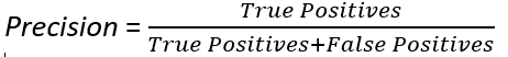
Precision

This expresses the ability of the algorithm to predict True Positives and avoid False Positives:

Recall

The ability to predict the records we want to find, the ones that were labelled belonging to the class we are looking at:

F1-score

F1 Score is the Harmonic Mean between Precision and Recall. The range for the F1 Score is [0, 1]. It tells how precise the classifier is (how many instances it classifies correctly), as well as how robust it is (it does not miss a significant number of instances).

The F1-score will be lower than the simple arithmetic means if one of the two measures is much lower than the other. And this is the reason why the F1-score is such a useful measure.

The above quality measures are defined for each individual class.

Binary Classification:

For a binary classification, we typically calculate these for the positive class. We want to find the cases belonging to that class. For a classification task where a bank wants to predict Fraud and No-Fraud transactions, the positive class would be Fraud as these are the ones we want to predict and find.

Cases belonging to the TP counter are the ones that are truly Fraud and where the classifier has predicted Fraud and FP cases would be No-Fraud cases, but the classifier has predicted Fraud.

Getting good Precision OR Recall is usually very easy, but getting good Precision AND Recall is often very hard. In general, we prefer classifiers with higher Precision and Recall scores. However, there is a trade-off between Precision and Recall; when tuning a classifier, improving the Precision score often results in lowering the Recall score and vice versa.

If the number of cases per class is not evenly distributed (also often referred to as not balanced), e.g. the number of cased labelled as Fraud is much smaller than the cases labelled as No-Fraud, Accuracy, Precision and Recall can be misleading if seen in isolation. Let us assume the Non-Fraud class is the majority class where, let’s say 90% of all cases are Non-Fraud and the classifier always predicts Non-Fraud. It would appear to be predicting correctly in 90% of all cases. This might look like a good result by just considering Accuracy as it is a measure for correctly predicting cases. Recall for the positive class, the ones we want to find would be 0%, but for the Non-Fraud class 100%. Precision would be 0% for our positive Fraud class, but 90% for the Non-Fraud class. For a bank it would mean that no fraudulent transactions are detected, this classifier would be rather useless. A far better approach is to combine these metrics into metrics like the F1-score and the macro-F1-score (see below).

Multi Class Classification:

For a multi class classification task, the target is a group of classes, like the one mentioned in 4.1, where we want to classify pictures of animals into the classes (cat, dog, mouse, fish), or a text narrative is classified into the SOC coding frame where the target has hundreds of classes. To be able to assess the overall quality of the classifier, we need to calculate the above measures for each class and combine them in either a Macro or Micro quality measure. This will give us a balanced view of the classifier’s ability to predict all classes.

Macro-Averaged:

The simplest way to combine the per-class measures into the respective Macro measures is to calculate the arithmetic mean for each of them:

As well as the above Macro-averaged measures, the averages might be weighted by the numbers of cases for each class. The quality measures are then called weighted-average or simply Weighted-Accuracy and so on.

Micro-Averaged:

The Micro-Averaged quality measures are also called:

• Micro-Accuracy
• Micro-Precision
• Micro-Recall
• Micro-F1-score

To calculate the Micro-Averages, we look at all the samples together. In a multi-class case, we consider all the correctly predicted cases to be True Positives, i.e. we add up TP = TP_Cat+ TP_Dog + TP_Mouse +TP_Fish

For the False Positives we have to count all the prediction errors. A photo of a cat that is predicted to be a fish, is a false prediction. It is a False Positive (FP) for the fish class but also a False Negative (FN) for the cat class, adding all these up, we end up with FP =FN. More broadly, each prediction error (X is misclassified as Y) is a False Positive for Y, and a False Negative for X.

And this implies that:

Micro-F1 = Micro-Precision = Micro-Recall = Micro-Accuracy

6. Classification and Coding Pilot Studies

At the time of writing this report, reports on 8 ML projects were submitted, see Table 3. Of these, 3 went either into production during this UNECE project or had already been operationalised when the project started, these are from StatsCanada, Statistics Norway and the US Bureau of Labor Statistics (BLS).

Table 3 – List of Pilot Studies

Table 4 – Steps/Features/Algorithm/Technology

The above Table 4 shows that the number of features used in the available data sets is typically rather small with the exception of the pilot study from Mexico where 15 features were used. This table also shows that the processing power used for ML training and prediction is typically that of a desktop or laptop computer. The exceptions are the two already operationalised solutions from Norway and BLS that use neural networks. Statistics Norway use Google Cloud and BLS use 4 GPUs with 3584 cores each.

Results of the individual pilot studies are shown in Table 5.

Table 5 – Results/Status/Future

7. Value added by Classification and Coding using ML in the production of official statistics 

The expectation on Machine Learning is to automate many traditional and manual processes inherent in the production of official statistics and manual Classification and Coding is one of them. The manual process is lengthy, resource hungry and can be prone to errors. Even Subject Matter Experts (SME) can give different outcomes to a C&C task as shown by the BLS report. 

The pilot studies from Canada and BLS have proven that data can be auto coded with ML to various degrees. Only predictions with high level of confidence are allowed to auto code in these solutions. The more mature the ML solution is, the more trust appears to be put into it to let ML take on more and more of the predictions.

As manual coding resources are freed up, possibly on an increasing scale over time, the cost of building, monitoring and keeping the ML solution current has to be accounted for just like a possibly expensive IT infrastructure. Data consistency will increase as manual coding is reduced.

The ML solution for Norway acts like an advisory to the human coding process. The human coder is given the 5 best ML predictions with their score and the option to either accept one of them or reject it. A similar approach is taken in BLS’ ML solution BLS where the human coders can reject suggested codes. However, BLS has shown that a suggested ML prediction is too easily accepted by the human coder, even if it is incorrect. While building their Gold Standard data set, they only used human coding from experts. These experts were not shown how other experts, humans or computers coded the case.

As ML takes on the task of auto coding big parts of the data sets, results become more rapidly available.

A financial gain was only reported by Statistics Norway and is expected to be over a 10-year period between 7,000,000 NOK and 17,000,000 NOK (650 000 € to 1 600 000 €).

8. Expected value added not shown 

The expectation that ML can fully replace the labour-intensive task of classification and coding straight after implementation has not been shown. The ML solutions from Canada and BLS only use the ML predicted classification if it is above a set confidence threshold. Predictions below that are ignored and completed manually instead; some solutions use these predictions as advisories to assist the human coders.

Tougher and rare cases still have to be coded by humans, but these manually coded cases can then be added as new training cases for the ML algorithm on a continuous basis. This in turn allows the ML solution to mature over time, which in turn should see a rise in the number of auto coded cases. This will help to balance the presence of labelled cases for the minority or difficult classes, but care has to be exercised not to create a bias in the training data. This cycle achieves an ever-increased timeline and resource savings. A simulation using the ML code and product description data shared by Statistics Poland clearly demonstrates this, albeit in a relatively simple context.

9. Best practises

These can be very subjective as this depends on the organisation’s expectations and the context in which the ML is to be used. The more successful pilot studies have shown that establishing a ‘Ground Truth’ or ‘Golden Data Set’ that is created manually and is deemed to be accurate and free of errors is of prime importance. A comparison between ML predictions, human coding and other legacy systems, such as rule-based systems, can only be clearly and credibly established when each is compared to a Golden Data Set in a statistically sound manner. Other pilot studies that are in the proof of concept (PoC) phase have stated that resources to build these data sets are not available.

The Neural Network techniques applied by BLS can provide better performance than the bag-of-words approaches that many others are using for text classification, but there are 2 big caveats. First, their knowledge of neural networks is advancing very rapidly, the best approach today will not be the best approach tomorrow and in fact even for BLS the neural network techniques are no longer consistent with the state of the start. Second, neural networks are very hard to use effectively. Just drop in a generic implementation will not get good results, the structure of the network needs to be adapted to the task using complicated tools like Tensorflow and Pytorch. Computationally expensive structures like recurrent neural networks are needed. That in turn means specialized computing resources (specifically very powerful GPUs) are needed which most organizations do not have and cannot easily acquire. Neural networks should be considered in more complex contexts (use case) and, preferably, after experimenting with less complex methods.

The first thing to try should not be neural network because it’s just so much harder. For most organizations, especially ones that are just starting out on their ML journey, the best approach is not the best approach available but rather a good approach that they have the resources to easily implement. That means some variation of bag-of-words, or even no or little pre-processing at all in order to try and experiment with ML. Good results can be achieved very quickly. To improve on these becomes more and more costly and time consuming. This depends on expectations, the use case and available resources. There will be a day in the not too distant future where that is no longer true, but it’s true for now.

Another approach could be to utilise cloud-based ML resources that do not carry the heavy capital burden compared to on-premises IT resources, but these come with other challenges, such as governance, security and simply trust to avoid the risk of disclosure of sensitive survey data.

10. Comparison of results

Prediction results vary between the pilot study reports. Different data, number of data records and varied quality of the ‘Ground Truth’ will be the reason for this as well as utilising different ML algorithms.

For example:

• INEGI use an in-house developed dictionary file of synonyms and a weighted assemble of ML algorithms for their classifications of the Economic activity.
• BLS is coding a wider range of variables, with a robust and advanced use of ML without much pre-processing.
• StatCan is coding a smaller number of variables, but excludes many classes based on predicted error.

The collaboration and code sharing during the pilot study phase of this project has helped and proven that, to some extent, proven solutions can be used in other settings (data, IT infrastructure, knowledge). However, there is no one solution that fits all Classification and Coding challenges. Not just resource constraints within IT environments and hardware resources enforce the use of less “expensive” ML algorithms, but also Data Science and ML knowledge as well. As that expertise and supporting resources build in an organisation, better results will be achieved.

The amount of available training data and the quality of the Ground Truth have just as much of an impact on ML results as the above-mentioned criteria.

11. Conclusions

It has been shown with collaboration and code sharing that an organisation that has basic ML knowledge can achieve very quickly good prediction results, even on small data sets. Classification and Coding is a prime example where ML can play a large part to speed up the production of official statistics. One must invest some time to get to that point; build and accumulate suitable training data to enable the ML algorithm to learn adequately; monitor its accuracy along the way; make appropriate use of ML predictions in combination with manual coding; and, allow data users time to gradually build their confidence in the data largely made or assisted with ML. It can make data better and more consistent.

It might save money, but that has to be seen on an individual basis. It is likely only viable (in terms of return on investment), if there is sufficient quality training data, computation capacity and ML expertise. There also has to be a predicted benefit of automation that outweighs investment in model development, maintenance over time and quality validation.